Mencari dan menghitung jumlah cell yang berisikan text/kata tertentu pada baris atau kolom excel

Menggunakan fungsi COUNTIF

Excel COUNTIF function
Fungsi COUNTIF 
Menghitung jumlah cell yang memiliki kata/karakter sesuai dengan kriteria yang kita tentukan
Formula
=COUNTIF (range, criteria)
Argumen
  • range - area baris dan kolom yang kita akan periksa
  • criteria - Kriteria yang akan kita hitung (text/karakter).
Catatan
Kriteria yang bukan berupa angka harus di ikuti dengan tanda kutip dua, untuk  kriteria yang berupa angka tidak perlu:

=COUNTIF(A1:A10,100) // count cells equal to 100
=COUNTIF(A1:A10,">32") // count cells greater than 32
=COUNTIF(A1:A10,"jim") // count cells equal to "jim"
=COUNTIF(A1:A10,"<"&B1) // count cells less than value in B1
The wildcard characters ? and * can be used in criteria. A question mark matches any one character and an asterisk matches any sequence of characters.

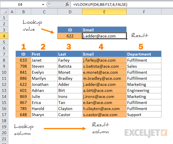
Membandingkan data dengan menggunakan fungsi VLOOKUP Excel

Excel VLOOKUP function

Penggunaan VLOOKUP 
Melihat/membandingkan nilai yang ada pada sebuah tabel dan mencocokkan nya dengan pada nilai yang ada di kolom pertama
Hasil 
Nilai/isi yang sesuai dengan tabel utama.
Formula 
=VLOOKUP (value, table, col_index, [range_lookup])
Argumen
  • value - nilai/data yang akan diperiksa pada kolom pertama.
  • table - tabel yang berisikan data.
  • col_index - kolom pada tabel yang digunakan sebagai acuan.
Catatan
VLOOKUP searches for a value in the first column of a table. At the match row, it retrieves a value from the specified column.
Use VLOOKUP when lookup values are located in the first column of a table with information organized vertically. Use HLOOKUP when lookup values are located in the first row of a table, and each "record" appears in a new column.
  • Range_lookup controls whether value needs to match exactly or not. The default is TRUE = allow non-exact match.
  • Set range_lookup to FALSE to require an exact match and TRUE to allow a non-exact match.
  • If range_lookup is TRUE (the default setting), a non-exact match will cause the VLOOKUP function to match the nearest value in the table that is still less than value.
  • When range_lookup is omitted, the VLOOKUP function will allow a non-exact match, but it will use an exact match if one exists.
  • If range_lookup is TRUE (the default setting) make sure that lookup values in the first row of the table are sorted in ascending order. Otherwise, VLOOKUP may return an incorrect or unexpected value.
  • If range_lookup is FALSE (require exact match), values in the first column of table do not need to be sorted.

Menghilangkan spasi pada awal dan akhir text pada cell excel

Seringkali saat kita melakukan copy dari data word atau test dari notepad dan paste ke Excel
ataupun saat menggunakan import data from text(csv to excel) kita mendapati text diawali dengan spasi atau di akhiri dengan spasi.

Mungkin hal ini adalah hal kecil yang tidak terlalu mengganggu user untuk melakukan olah data pada excel. tetapi akan menjadi masalah saat user akan menggunakan fungsi seperti lookup, exact, vlookup. dimana pembandingan data tidak dapat dilakukan karena adanya perbedaan spasi.
berikut cara mengatasi nya

Excel formula: Remove leading and trailing spaces from text

Generic formula 
=TRIM(text)
Penjelasan 
untuk menghilangkan spasi pada awal dan akhir text, anda dapat menggunakan fungsi Trim. dimana fungsiini akan mencari spasi pada awal dan akhir text dan menghilangkannya, menyisakan text yang kita butuhkan.
seperti contoh pada gambar,formula pada kolom C3 adalah:

=TRIM(B3)

TRIM dengan CLEAN

jika anda juga ingin menghilangkan karakter line breaks pada cells, anda dapat menambahkan fungsi CLEAN seperti berikut:

=TRIM(CLEAN(text))
Fungsi CLEAN akan menghapus karatker-karakter yang tidak perlu atau yang tidak ingin kita cetak seperti line breaks, dan akan menyisakan "cleaned" text. 

Masalah dengan karakter lainnya

Fungsi Clean tersebut tidak benar-benar bisa menghilangkan semua karakter karakter yang tidak kita butuhkan, seperti karakter-karakter khusus lainnya. dengan menambahkan fungsi SUBSTITUTE pada formula, anda dapat menghilangkan karakter spesifik. seperti contoh, menghilangkan non-breaking space:
=TRIM(CLEAN(SUBSTITUTE(B1,CHAR(160)," ")))
Selamat mencoba.

How to block facebook in Mikrotik using L7 Protocols (Layer 7)

This tutorial consists of two parts:
1- Block facebook website for everyone on local network.
2- Allow facebook for specific host(s) and block for others on local network.

1- Block facebook website for everyone on local network.
First we check that Facebook is currently working on our local network or not?

Check the IP address of our client?

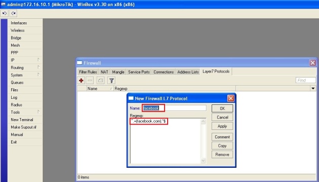
We need to create new Regexp rule at Layer7 Protocols, in order to block the facebook for our local network.
To achieve this goal, please follow these steps:


^.+(facebook.com).*$
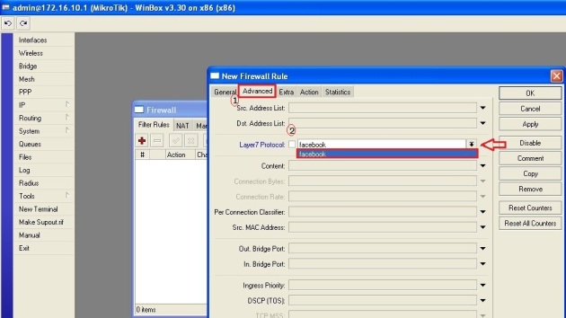
Now, we need to create Filter Rule, using these steps:

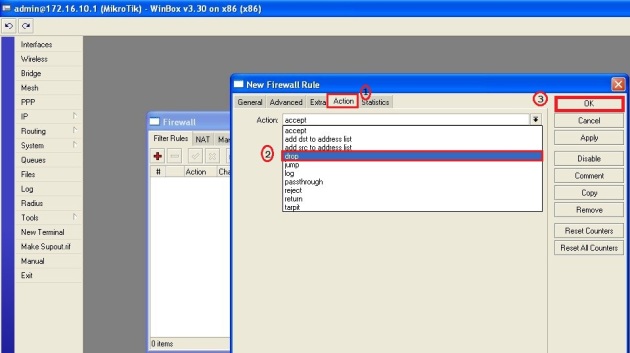
Now test the rule, that we just created:

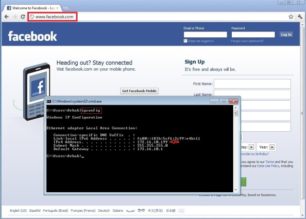
Try also on 2nd client (172.16.10.199/24):
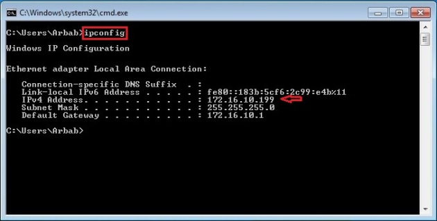

Check that it only block facebook or other websites also?

Oh yes, our rule is working perfectly :)
2- Allow facebook for specific host(s) and block for others on local network.
Now, we want to allow facebook for 2nd client (172.16.10.199/24) but still want to block it for other host(s).
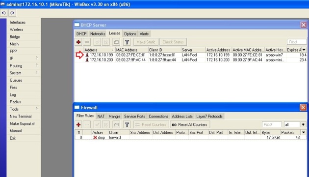
To accomplish this goal, we need to create a second Filter rule, to do this, please follow these steps:
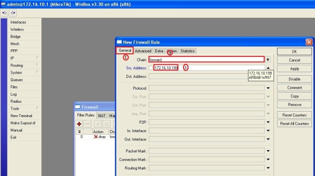

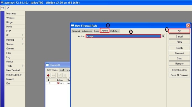
Move this rule at the top:
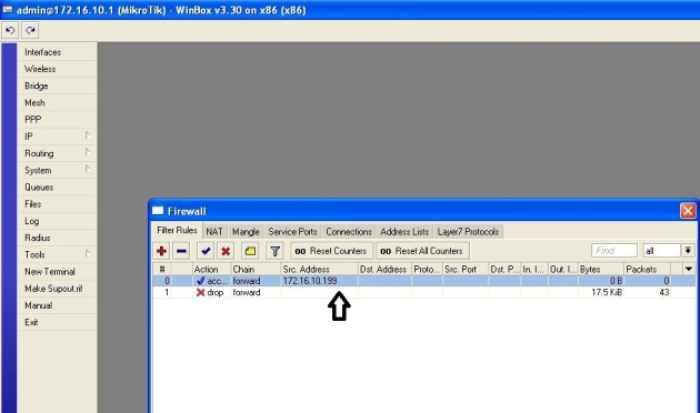
Test this rule on 2nd client (172.16.10.199/24):
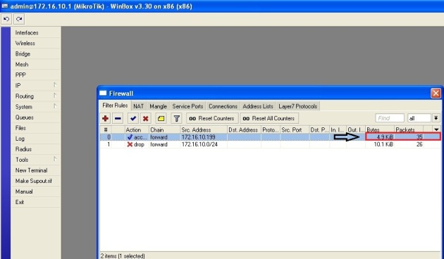
Verify the rule on Mikrotik:
Verify that, facebook is still blocked for other host(s) on the local network:
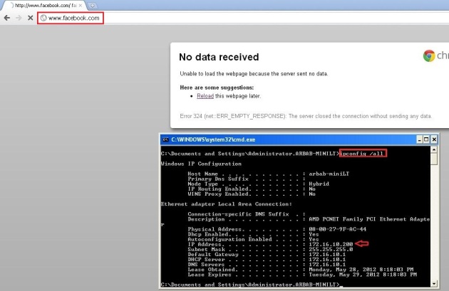
Verify the rule(s) on Mikrotik:
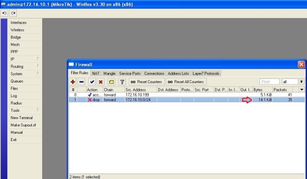
Drop packets rate are incremented!
We can do the same for youtube or any other website!